How much do you know by digging deep into the design elements of smart cars?

Overview

This article refers to the address: http://

From the navigation operation of the Boeing 747, the GPS navigation system that the car uses every day, to the treasure hunt to find a treasure hidden deep in the forest, GPS technology has quickly integrated into a variety of applications.

As innovative technologies continue to improve the performance of GPS receivers, the relevant technical features are becoming more and more complete. Today, the software can even build GPS waveforms to accurately simulate actual signals. In addition, the instrument bus technology has been continuously improved, and the PXI instrument control function can be used to record and play real-time GPS signals.

Introduction

Since GPS technology has become popular in the general commercial market, many designs are focused on improving related features, such as:

1) Reduce power consumption

2) Looking for weak satellite signals

3) Faster capture times

4) More precise positioning function

Through this application note, you will be able to learn how to perform multiple GPS receiver measurements: sensitivity, noise figure, positioning accuracy, first positioning time, and position error. This technical document is intended to give engineers a thorough understanding of GPS measurement techniques. For engineers who are new to GPS receiver measurement, they can get a glimpse of common measurement tasks. If the engineer already has relevant experience in GPS measurement, you can also get a preliminary understanding of the new instrument control technology through this technical document. This application note will be divided into the following paragraphs:

1. The basis of GPS technology

2.GPS measurement system

3. Overview of common measurements

Sensitivity

b. First positioning time (TTFF)

c. Positioning accuracy and repeatability

d. Tracking accuracy and repeatability

Each paragraph will provide several practical tips and tricks. More importantly, readers can compare their results with those obtained by GPS receivers. Through your own results, the results of the receiver, and the results of theoretical measurements, you can further examine your measurement data.

Introduction to GPS navigation system

The Global Positioning System (GPS) is a space-based radio navigation system developed by the US Air Force. Although GPS was originally developed as a military positioning system, it also has an important impact on the people. In fact, you are currently using GPS receivers in vehicles, ships, and even mobile phones. The GPS navigation system consists of 24 sets of satellites, each transmitting multiple signals in the L1 and L2 bands. Through the 1.5542 GHz L1 band, each group of satellites generates a spread spectrum signal of 1.023 Mchips BPSK (binary phase key shift). The spread spectrum sequence uses a virtual random number (PN) sequence called a C/A (coarse acquisition) code. Although the spread spectrum sequence is 1.023 Mchips, the actual signal data transmission rate is 50 Hz [1]. In the original deployment of the system, the general GPS receiver can reach an accuracy error of 20 to 30 meters or more. This error is due to the random frequency error attached by the US military for security reasons. However, this is called the Selective availability error signal source and was cancelled on May 2, 2000. Today, the maximum error of the receiver is no more than 5 meters, and the general error has been reduced to 1 to 2 meters.

Whether in the L1 or L2 (1.2276 GHz) band, GPS satellites produce so-called "P-code" satellite signals. This signal is a modulated signal of 10.23 Mbps BPSK, and the PN sequence is also used as the spreading code. The military uses the transmission of the P code to perform more precise positioning operations. In the L1 band, the P code is an 90-degree transmission of the Outofphase through the C/A code to ensure that the two signal codes can be measured on the same carrier [2].P code in the L1 band. Up to -163dBW of signal power; up to -166dBW in the L2 band. Relatively speaking, if the C/A code on the Earth's surface, the minimum broadcast power of -160dBW can be achieved in the L1 band.

GPS navigation signal

For the C/A code, the navigation signal is composed of 25 frames of data, and each frame contains 1500 bits [2]. In addition, each group of frames can be divided into 5 groups of 300 bits. Sub-framework. When the receiver captures the C/A code, it takes 6 seconds to capture 1 sub-frame, that is, 1 frame must take 30 seconds. Please note that in fact, some of the more in-depth measurement operations can actually take 30 seconds to capture the complete framework; we will discuss it later. In fact, 30 seconds is only the average minimum time to capture the full frame; the system's first positioning time (TTFF) often exceeds 30 seconds.

In order to perform positioning operations, most receivers must update the information of the satellite ephemeris (Almanac) and the ephemeris (Ephemeris). This information is included in the signal data transmitted by the satellite, and each sub-frame also contains a proprietary information set. In general, we can identify the information contained in the sub-frame by the category of the sub-frame [2][7]:

Sub-frame1: contains timing correction, accuracy, and the operation of the satellite

Sub-frame2-3: contains accurate orbital parameters to calculate the exact position of the satellite

Sub-frames 4-5: Contains rough satellite orbit data, timing corrections, and operational information.

The receiver must pass the information of the satellite ephemeris and the ephemeris to be able to perform the positioning operation. Once the true distance of each group of satellites is obtained, the high-order GPS receiver will return the position information through a simple triangulation algorithm. In fact, the ability to integrate Pseudorange and satellite position information will allow the receiver to accurately identify its location.

Whether using a C/A code or a P code, the receiver can track up to 4 sets of satellites for 3D positioning. The process of tracking satellites is extremely complicated, but in simple terms, the receiver will estimate its position through the distance of each group of satellites. Since the signal travels at the speed of light (c), or 299,792,458 m/s, the receiver can calculate the distance from the artificial satellite by the following equation, which is called "Pseudorange":

Equation 1. "Psedorange" is a function of time interval [1][4]

The receiver must decode the signal data transmitted by the satellite to obtain the positioning information. Each satellite broadcasts its location, and the receiver follows the difference in virtual distance between each set of satellites to determine its exact location [8]. The triangulation used by the receiver, 2D positioning can be performed by 3 sets of satellites; 3 sets of satellites can perform 3D positioning.

Setting up a GPS measurement system

The main product of the GPS receiver is a set of RF vector signal generators that can simulate GPS signals. In this application note, the reader will learn how to use the NI PXI-5671 and NI PXIe-5672RF vector signal generators for measurement purposes. This product can be paired with the NI GPS tool set to simulate 1 to 12 GPS satellites.

The complete GPS measurement system should also include a variety of different accessories for optimum performance. For example, an external fixed attenuator (Attenuator) can improve the power accuracy and noise floor performance. In addition, some receivers may also require a DC blocker depending on whether the receiver supports its direct input DC bias (Bias). The following picture shows the complete system of GPS signal generation:

Figure 1. Program diagram of the GPS generation system

As shown in Figure 1, when testing GPS receivers, external RF attenuation (Padding) of up to 60 dB is often used. A fixed attenuator provides at least two advantages of a measurement system. First, the fixed attenuator ensures that the noise floor of the test excitation is below the thermal noise floor of -174dBm/Hz. Second, fixed attenuators can also improve power accuracy because the signal level can be calibrated through a high-accuracy RF power meter. Although only 20dB of attenuation is required to meet the noise floor requirements, higher power accuracy and noise floor performance can be achieved with 60 to 70dB attenuation. The RF power calibration will be discussed later, while Figure 2 preemptively illustrates the effect of attenuation on the noise floor performance.

Figure 2. Comparison of instrument power required for different attenuations

As shown in Figure 2, the attenuation can be used to attenuate noise, and is not limited to a thermal noise floor of -174 dBm/Hz.

RF vector signal generator

When selecting an RF vector signal generator, the NI abVIEW GPS tool set supports both the NI PXI-5671 and NI PXIe-5672RF vector signal generators. Although the two adapter cards can generate GPS signals, the NI PXIe-5672 vector signal generator is favored because of its fast PCI Express bus speed and immediate IF equalization. Both adapters feature a 6MB/s total data rate and a 1.5MS/s (IQ) sampling rate to stream GPS waveforms from the disk.

Although PXI controller hard drives can easily maintain this data transfer rate, NI recommends using an external disk for additional storage capacity. The following picture shows a common PXI system with NI PXIe-5672:

Figure 3. PXI system with NIPXIe5672VSG and NIPXI-5661VSA

The GPS tool set creates waveforms up to 12.5 minutes (25 frames) during the full navigation signal. At a sampling rate of 6MB/s, the maximum file size is approximately 7.5GB. Due to the waveform file size described above, all waveforms can be stored in one of several hard disk options. These waveform storage resource options include:

o Hard disk of PXI controller (recommended to use 120GB hard disk upgrade)

o External RAID devices such as HDD8263 and HDD8264

o External USB2.0 hard drive (tested by Western Digital Passport)

All of the above hard disk settings can support continuous data streaming operations over 20MB/s. Therefore, any storage option can simulate GPS signals and record and play them. In a later paragraph, the integration of the simulation and recording of the GPS waveform will be described, and the Characterization of the GPS receiver performance will be performed.

Establish a simulated GPS signal

Since the GPS receiver transmits data through the antenna and obtains satellite ephemeris and ephemeris information; of course, the simulated GPS signal also needs this information. Satellite ephemeris and ephemeris information, both represented by text files, provide information on satellite position, satellite altitude, machine status, and orbits. In addition, in the process of establishing the waveform, M must also select custom parameters such as day of the week (TOW), position (longitude, latitude, altitude), and the receiver rate of the simulation. Based on this information, the tool set will automatically select up to 12 sets of satellites, calculate all Doppler shift and Pseudorange information, and then generate the desired baseband waveform. In order to get started as soon as possible, the toolkit installer also includes sample satellite ephemeris and ephemeris files. In addition, it can be downloaded directly from the following websites:

. Almanac information (The Navigation Center of Excellence) http://navcen.uscg.gov/gps/almanacs.htm

. Ephemeris information (NASA Goddard Space Flight Center) http://cddis.gsfc.nasa.gov/gnss_datasum.html#brdc

Through custom satellite ephemeris and ephemeris files, GPS signals can be created for specific dates and times, even back a few years ago. Please note that when selecting these files, you must select the file corresponding to the date. In general, satellite ephemeris and ephemeris information are updated daily, so when selecting a specific time and date, you should also select the same day file. The downloaded ephemeris files are often in a compressed "*.Z" format. Therefore, the file must be decompressed before using the GPS tool set.

As long as you use the "Automatic mode" in the tool group, you can include most GPS module jobs, and you can calculate the Doppler and random distance information through programming. Of course, this function also provides manual mode. In Manual mode, the user can individually specify information for each group of satellites. Figure 4 shows the input parameters provided by these two modes of operation.

1LLA(longitude,latitude,altitude)

Figure 4. Default values ​​for the GPS Tool Set Auto and Manual modes

Please note that the tool set will force the GPS TOW to be within the possible range of values ​​based on the specified ephemeris file. Therefore, if the selected value is outside the range of the ephemeris file, the tool set will automatically be set to the closest The value and remind the user. The “niGPS Write Waveform To File” sample program creates a GPS baseband waveform (automatic mode), and its human-machine interface is shown below.

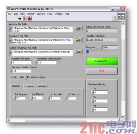
Figure 5. A simple sample program to create a GPS test waveform.

Please note that certain measurement jobs will determine the type of file the GPS test is built by the user. For example, when measuring receiver sensitivity, a single satellite will be simulated. On the other hand, the measurement of the positioning job (such as TTFF and positional accuracy) is required, and the GPS signals used will simulate multiple sets of artificial satellites. Based on the above requirements, the sample program of the NIGPS tool set will include both unit star and multi-satellite simulation functions.

Record GPS signals in the air

When creating GPS waveforms, their unique and increasingly common way is to draw directly from the air. In this test, we used a vector signal analyzer (such as the NI PXI 5661) to record the signal, and then generate a recorded signal through a vector signal generator such as the NI PXIe-5672. Since the actual signal impairments can also be captured when recording GPS signals, the receiver can be further informed about the operation of the receiver in the deployment environment.

The GPS signal in the air can be captured in a very direct way. In the RF recording system, we use a suitable antenna and amplifier with a PXI vector signal analyzer and hard disk to capture continuous data for up to several hours. For example, a set of 2TB RAID arrays can record up to 25 hours of GPS waveforms. Since this technical document will not discuss the special techniques of streaming, if you need the relevant sample program code, please go to: http:// Through the following paragraphs, you can understand how it should be. Set the appropriate RF front-end for the RF recording and playback system.

Different types of wireless communication signals require different bandwidths, central frequencies, and gains. In terms of GPS signals, the basic system requirements are to record the 2.062 MHz RF bandwidth at a central frequency of 1.57542 GHz. According to this bandwidth requirement, at least 2.5MS/s (1.25x2MHz) sampling rate must be achieved. Note: The 1.25 multiplier here is based on the PXI-5661 Digital Down Converter (DDC) in the Decimation phase of the Roll-off filter.

In the test scenario described below, we used a 5MS/s (20MB/s) sampling rate to capture the full bandwidth. Since the standard PXI controller hard disk can achieve 20MB/s or higher data traffic, GPS signals can also be streamed to the disk without using an external RAID. However, for two reasons, we still recommend using an external hard drive. First, an external hard drive can increase overall data storage and record multiple sets of waveforms. Second, the external hard drive does not impose an additional burden on the PXI controller's hard drive. In the test operation described below, we use a set of USB2.0 external hard drives. The drive is a 320GB Western Digital Passport with a 5400RPM hard drive speed. In our test operation, the general reading speed is about 25~28MB/s. Therefore, this hard disk can be used for both GPS waveform data stream simulation (6MB/s) and recording (20MB/s).

The most special feature of GPS signal recording is the selection and setting of the appropriate antenna and low noise amplifier (LNA). A common peak power of -120~-110dBm (here -116dBm) can be found in the L1GPS band through a passive passive patch antenna. Since the power of the GPS signal is extremely small, amplification must be performed so that the vector signal analyzer can capture the full dynamic range of the satellite signal. Although there are several ways to apply the appropriate gain to the signal, we found that the best results can be achieved with an active GPS antenna with the NIPXI-5690 Pre-amplifier. If two sets of LNAs with up to 30dB gain are connected in series, the total gain can reach 60dB (30+30). Therefore, the peak power that the vector signal analyzer can measure will increase from -116dBm to -56dBm. The following figure shows an example system for this setting:

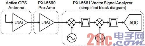
Figure 6. GPS receiver and LNA in series.

Please note that one of the prerequisites for the operating system is the active GPS antenna. Active GPS antenna consists of a set of planar antennas and a set of LNAs. This antenna typically requires a DC bias voltage of 2.5V to 5V and can be purchased for off-the-shelf products for only $20. For the sake of simplicity, we use a set of antennas with a set of SMA connectors. As we will see in the following paragraphs, the first set of LNA noise patterns at the RF front end is extremely important; this pattern will confirm the instrumentation of the recording operation and whether it poses the lowest noise to the wireless signal. Also note that the vector signal analyzer in Figure 6 is a simplified icon. The actual PXI-5661 is a 3-stage Super-heterodyne vector signal analyzer, which is more complicated than shown in the figure.

If 60dB is applied to the wireless signal, a peak power of about -60~-50dBm can be obtained in L1. If the VSA is set in the Swept spectrum mode and the overall spectrum is analyzed, the power in band outside the L1 band (FM and mobile) will also be found, which will be stronger than the GPS signal. However, the peak power of the out-of-band signal generally does not exceed -20 dBm and will be filtered through one of the VSA's multiple sets of band pass filters. One of the easiest ways to view the RF front end of a recording device is to open a sample program for the RFSA demonstration panel. Through this procedure, the RF spectrum can be presented in the L1GPS band. Figure 7 shows the common spectrum. Please note that this spectrum screenshot is obtained outside the GPS center frequency. The active GPS antenna and PXI-5690 preamplifier achieve a total gain of 60dB.

Center frequency: 1.57542GHz

Spreading frequency (Span): 4MHz

RBW: 10Hz

Average: RMS, 20Averages

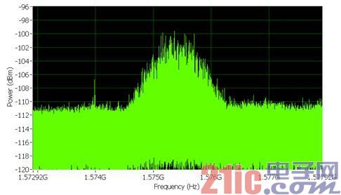
Figure 7. GPS can be rendered in the spectrum with only a small resolution bandwidth (RBW)

Here we use the RF recording and playback LabVIEW sample program mentioned above; set the reference level of -50dBm, the center frequency of 1.57542GHz, and the IQ sampling rate of 5MS/s. The following figure shows the human interface of the setup example:

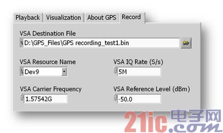
Figure 8. Human-machine interface for RF recording and playback examples.

The maximum recording time of the GPS signal will depend on the sampling rate and the maximum storage capacity. If you use a 2TB capacity Raid disk array (the largest disk supported by Windows XP), you can record up to 25 hours of signal through the 5MS/s sampling rate.

Set the RF front end

Since the series LNA provides 60dB of gain, the user can greatly increase the power of the vector signal analyzer front end. In our measurement operation, a gain of 60dB is sufficient to increase the peak power from -116dBm to -56dBm. With a gain of 60dB (with a noise figure of 1.5dB), the noise power of the signal will be –112dBm/Hz (- 174+ gain + F). Therefore, the signal-to-noise ratio (SNR) that can be achieved is up to 56.5dB (-56dBm + 112.5dBm), which is also lower than the actual instrument dynamic range. It can be seen that if there is a dynamic range of 80 dB, the VSA will record the maximum SNR without the noise of the wireless signal.

When recording any wireless signal, the reference level can be set at least 5 dB above the normal peak power to account for any signal strength anomalies. In some cases, although this step will reduce the effective dynamic range of the VSA, the GPS signal will not be affected. Since the maximum ideal SNR of the GPS signal at the antenna input is 58dB (-116+174), there is no point in recording a dynamic range of more than 58dB in the VSA. Therefore, we can even “discard” the instrument's dynamic range by more than 10dB without affecting the quality of the recorded signal (in this bandwidth, the PXI-5661 will provide a dynamic range better than 75dB).

Since the appropriate reference level must be set, it is equally important to properly set the RF front end of the recording device. As mentioned earlier, an active GPS antenna is recommended for optimal RF recording data. Since the active antenna has a built-in LNA that provides up to 30dB of gain with a low noise figure, DC bias can also be supplied. A variety of biasing methods will be described below.

Method 1: Active antenna powered by GPS receiver

The first method is to supply the active antenna with a DC bias "T". In this example, we apply a DC signal (this is 3.3V) to the DC埠 of the bias "T", and "T" applies the appropriate DC offset to the active antenna. Please note that the DC power requirement of the active antenna will be used here to determine whether or not to apply the exact DC voltage. The figure below shows the relevant link situation.

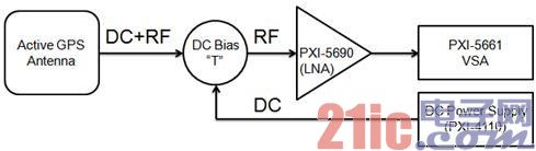
Figure 9. Powered to Active GPS Antenna Using DC Bias "T"

As can be seen in Figure 9, the PXI-4110 can be programmed with a DC power supply to supply a DC bias signal. While several off-the-shelf power supplies (which also include lower-priced power supplies) can be used in this application, we use the PXI-4110 to simplify the job. Similarly, the existing common biaser (Bias tee) can operate up to 1.58 GHz, and the biasing device used here is available from

Method 2: Powering the receiver to the active antenna

The second method of supplying power to the active GPS antenna is through the receiver of the antenna itself. Most off-the-shelf GPS receivers use a single port to power the active GPS antenna, and this port is also biased by a suitable DC signal. If the active GPS receiver is integrated with a splitter and a DC blocker, it can be powered to the active LNA and only the signals obtained by the GPS receiver are recorded. The figure below is the correct way to connect:

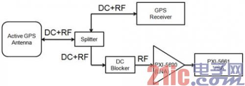
Figure 10. Through the DC Blocker, the GPS signal can be recorded and analyzed.

As shown in Figure 10, the DC bias of the GPS receiver is used to supply power to the LNA. Please note that since the receiver can be observed, the relevant characteristics of the receiver, such as speed and accuracy Dilution, can be observed. Method 2 is especially useful for driver testing.

Noise figure calculation of series figure

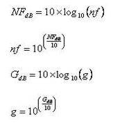
To calculate the total amount of noise of the recorded GPS signal, simply find the noise figure of the overall RF front end. In general, the noise figure of the entire system is often affected by the first set of amplifiers in the system. In all RF components or systems, the noise figure can be considered as the ratio of SNRin to SNRout (see: Noise Factor of Measurement Technology). When recording GPS signals, you must first find the noise figure of the overall RF front end.

When performing series noise figure calculation, it must first convert each noise figure and gain into a linear equation; the so-called "Noise factor". When calculating the noise figure of the system with the RF component in series, the noise factor of the system can be found first and then converted to the noise figure. Therefore the noise figure of the system must be calculated using the following equation:

Equation 2. Noise figure calculation operation of series RF amplifier [3]

Note that since the noise factor (nf) and the gain (g) are linear rather than logarithmic, they are represented in lowercase. The following equations for gain and noise figure, from linear to logarithmic (and vice versa):

Equation 3 to Equation 6. Linear/Logarithmic Conversion of Gain and Noise Figure [3]

Active GPS antennas with built-in low noise amplifiers (LNAs) typically provide 30dB of gain with a noise figure of approximately 1.5dB. In the second phase of the instrumented recording operation, the NIPXI-5690 provides 30dB of additional gain. . Due to its high noise figure (5dB), the second set of amplifiers will only generate very little noise into the system. In the teaching implementation, the noise factor can be calculated using Equation 2 for the complete RF front end of the recorder control operation. The gain and noise figure values ​​are as shown below:

Figure 11. Noise figure and factor for the first two components of the RF front end.

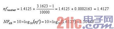
According to the above calculation, you can find the overall noise factor of the receiver:

Equation 7. Series noise figure of the RF recording system

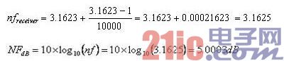
To convert the noise factor to a noise figure (in dB), Equation 3 can be applied to obtain the following results:

Equation 8. The noise figure of the first set of LNAs will affect the noise figure of the receiver.

As shown in Equation 8, the noise figure of the first set of LNAs (1.5 dB) will affect the noise figure of the entire set of measurement systems. Through the VSA related settings, the noise floor of the instrument can be lower than the noise level of the input excitation, so the recording operation performed by the user will only cause 1.507dB noise to the wireless signal.

Signaling to the GPS receiver

Since a variety of receivers can use appropriate software to allow users to present information such as longitude and latitude, a more standardized way to perform automated measurement operations is required. Fortunately, a number of receivers are currently available to signal the PXI controller through the well-known NMEA-183 protocol. In this way, the receiver will continuously transmit the relevant commands through the serial or USB cable. In NI LabVIEW, all instructions can be converted to syntax to return satellite and location information. The NMEA-183 protocol supports six basic instructions and each represents proprietary information. These instructions are as shown in the following table.

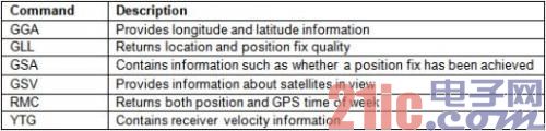
Figure 12. Overview of the basic NMEA-183 instructions

In terms of actual test needs, GGA, GSA, and GSV instructions should be most practical. It is worth mentioning that the GSA command information can be used to know whether the receiver can meet the positioning operation needs, or can be used for Time To First Fix (TTFF) measurement. When performing highly sensitive measurements, the C/N (Carrier-to-noise) ratio can actually be returned for the satellite being tracked using the GSV command.

Although it is not possible to elaborate on the MNEA-183 protocol, you can go to other websites to find all the instruction information, such as: http://#RMC. In LabVIEW, these instructions can be transparent. The NI-VISA driver converts its syntax.

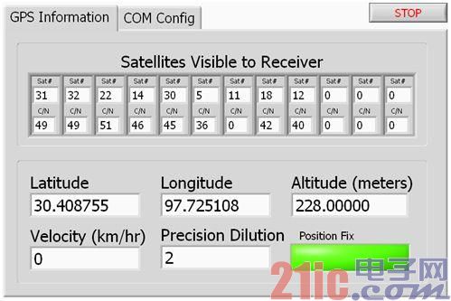
Figure 13. LabVIEW example using the NMEA-183 protocol

GPS measurement technology

There are a variety of measurement operations available to characterize the performance of GPS receivers, and several common measurements can be applied to all GPS receivers. This chapter will explain the theory and implementation of performing measurements such as sensitivity, first positioning time (TTFF), positioning accuracy/reproducibility, and positioning uncertainty (Uncertainty). It should be noted that there are many different ways to verify the positioning accuracy and perform the receiver tracking function test. Although there are a number of basic ways to follow, it is not possible to summarize everything.

Sensitivity measurement job introduction

Sensitivity is one of the most important measurement tasks for GPS receiver functions. In fact, for a number of mass-produced GPS receivers, it is limited to the RF measurements performed in the final production test. In more depth, the sensitivity measurement is “the lowest satellite power strength at which the receiver can track and receive satellite positioning information above”. It is generally believed that GPS receivers must be connected in series with multiple sets of LNAs to achieve extremely high gains in order to amplify the signal to the appropriate power level. In fact, although the LNA can increase the signal power, it may also reduce the SNR. Therefore, when the RF power of the GPS signal decreases, the SNR will also decrease, and finally the receiver cannot track the satellite.

A variety of GPS receivers can specify two sets of sensitive values: Acquisition sensitivity and Signal tracking sensitivity [9]. As literally, the sensitivity is "the lowest position that the receiver can locate." Power intensity". Conversely, the signal tracking sensitivity is "the receiver can track the lowest power intensity of each satellite."

In terms of basic concepts, we can define sensitivity as "the lowest power level at which the wireless receiver produces the required minimum bit error rate (BER)." Since the BER is closely related to the carrier-to-noise (C/N) ratio, the sensitivity is generally determined by the known receiver input power level to obtain the desired C/N value.

Please note that the C/N values ​​of each group of satellites can be obtained directly from the chipset of the GPS receiver. There are currently several ways to calculate this value, and some receivers calculate the date of the message (Messagedate) and get an approximate value. The new GPS receiver typically achieves a C/N peak of 54 to 56 dB-Hz when simulated by high power test excitation. Since even a cloudless clear sky, the GPS receiver may also obtain a C/N value of 30~50dB-Hz; therefore, the C/N limit is still within the normal range. Generally, the GPS receiver must reach the minimum C/N ratio to meet the 28~32dB-Hz positioning (capture sensitivity) range. Therefore, the sensitivity of some special receivers can be defined as "the lowest power strength required by the receiver to produce the lowest C/N ratio."

In theory, single or multiple sets of satellite test excitations can measure sensitivity. In practice, measurement operations are often performed in a single satellite mode because the required RF power can be easily and stably generated. By definition, sensitivity is the lowest power strength at which the receiver returns the minimum C/N ratio. In the following discussion, it can be found that the sensitivity of the receiver is very dependent on the noise figure of the RF front end.

In Equation 9, the sensitivity can be expressed as a function of the C/N ratio and the noise figure. For example, the minimum C/N required for position tracking is 32 dB-Hz, and a receiver with a noise figure of 2 dB will have a sensitivity of -140 dBm (-174+32+2). However, when testing a baseband transceiver separately, the first set of LNAs is often overlooked. The general receiver is shown below:

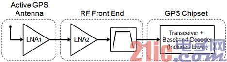
Figure 14. GPS receivers tend to cascade multiple sets of LNAs [6]

As shown in Figure 14, the general GPS receivers are connected in series with multiple sets of LNAs to provide high efficiency gain for GPS signals. As mentioned earlier, the first set of LNAs will determine the noise figure of the entire system. In Figure 14, we assume that LNA1 has a gain of 30dB and a NF of 1.5dB. In addition, we assume that the entire RF front end has 40dB of gain and 5dB of NF. Then note that the noise power after LNA2 will exceed -174dBm/Hz. Thermal noise, so the Bandpass filter will both attenuate the signal and noise. This will have little impact on SNR. Finally, we assume that the GPS chipset can produce 40dB of gain and 5dB of noise figure. The noise figure of the entire system can be calculated as:

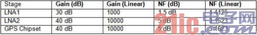
Figure 15. Gain and NF for linear and logarithmic modes

According to the above calculation, you can find the overall noise factor of the receiver:

Equations 10 and 11. The noise figure of the first set of LNAs will affect the noise figure of the receiver.

Looking through Equations 10 and 11, if the GPS receiver is connected to an activated antenna, its noise figure is about 1.5 dB. Please note that we have omitted the third condition in the relevant noise figure equation. Since this value is extremely small, it can basically be ignored.

In some cases, the GPS receiver's operating antenna will be paired with the built-in LNA. Therefore, the test point will ignore the receiver's first set of LNAs. This will result in a noise figure through the second set of LNAs, and often It is also larger than the noise figure of the first group of LNAs. If LNA1 is removed, the noise figure of LNA2 can be derived from the following equation.

Equations 12 and 13. Receiver noise figure obtained by removing the first set of LNAs

As shown in Equations 12 and 13, removing the LNA with the best noise figure will greatly affect the noise figure of the entire set of receivers. Please note that although the calculation example of this "common" GPS receiver noise figure is purely theoretical, it is still of importance. Since the C/N ratio presented by the receiver is inseparable from the noise figure of the system, the noise figure of the system can help us set the appropriate C/N test limits.

Single satellite sensitivity measurement

After understanding the basic theory of sensitivity measurement, the individual procedures for the actual measurement will then be performed. The general test system sends the simulated L1 single satellite carrier to the DUT's RF communication port through direct connection. In order to obtain the C/N ratio, we communicate the receiver settings via the NMEA-183 protocol. In LabVIEW, you can read the maximum satellite C/N value by simply connecting 3 GSV commands in series.

According to the GPS specification, if a single L1 satellite is located on the surface of the Earth, its power should be no less than -130dBm [7]. However, consumer demand for indoor and outdoor GPS receivers has further depressed the test limits. In fact, a variety of GPS receivers can achieve a minimum -142dBm position tracking sensitivity, with a minimum -160dBm signal tracking. At the normal operating point, most GPS receivers can quickly lock signals below 6dB, so our test excitation uses an average RF power of -136dBm.

To achieve the best power accuracy and noise floor performance, it is recommended to use an external attenuation for the output of the RF vector signal generator. In most cases, an external attenuation of 40dB~60dB allows us to get closer to the linear range (power ≥-80dBm) and operate the generator properly. Since the set attenuation of each group of receivers is not fixed, the system must be calibrated first to determine the correct power for the test excitation.

In the calibration procedure, we can consider: 1) the peak-to-average ratio of the signal, the difference between the various parts of the attenuator, and the possible insertion loss (Insertionl oss) of any wiring operation. In order to calibrate the system, the connection should be disconnected from the DUT and then connected to an RF vector signal analyzer (such as the PXI-5661).

PartA: Single Satellite Calibration

When performing sensitivity measurements, the accuracy of the RF power intensity is one of the most important characteristics of the signal generator. Since the receiver can obtain a C-N value of 0 digital accuracy (such as 34dB-Hz), the sensitivity measurement in the production test can reach a power accuracy of ±0.5dB. Therefore, we must ensure that our instrument control functions must achieve at least equal or more performance. Since general RF instrumentation is designed for a wide range of power intensities, frequency ranges, and temperature conditions, the repeatability of measurements should be much higher than the performance of a particular instrument when performing basic system calibration. The following sections will further illustrate two methods for ensuring RF power accuracy.

Method 1: Single Passive RF Attenuator:

Although the external attenuation is used to ensure that the GPS signal generation operation can achieve the best noise density, only 20dB of attenuation is actually required to ensure the noise density is lower than -174dBm/Hz. When using a 20dB fixed plate (Pad), Simply set the instrument to an RF power level of more than 20 dB. To achieve the -136dBm target, the instrument should be programmed to -115dBm (assuming 1dB of line insertion loss) and connect the 20dB attenuator directly to the generator's output. The RF power achieved will be -136dBm, but still has additional uncertainty.假设20dB的固定板具有±0.25dB的不确定性，且RF产生器亦于-116dBm具有±1.0dB的不确定性，则整体的不确定性将为±1.25dB.因此，虽然方法1最为简单且不需进行校准，但由于系统中的多项组件均未经过校准，因此可能接着发生不确定性。请注意，造成仪器不确定性最主要的原因之一，即为电压驻波比(Voltage standing wave ratio，VSWR)。因为被动式衰减器是直接连至仪器的输出，所以反射回仪器的驻波即为实际衰减。由于降低了功率的不确定性，因此可提升整体功率的精确性。

请注意，此处亦使用高效能VNA确实测量被动衰减器。透过此测量装置，即可于±0.1dB的不确定性之内，决定所要套用的衰减。

方法2：经过校准的多组被动衰减器

校准RF功率的第二种方法，即是使用高精确度的RF功率计(高于±0.2dB的精确度，并最低可达-70dBm)搭配多款固定式衰减器。因为我们是以固定频率，与相对较小的功率范围操作RF产生器，所以可有效修正由产生器造成的任何错误。此外，由于被动衰减器是以固定频率进行线性动作，因此亦可校准其不确定性。在方法2中，主要即必须确保产生系统可达到最佳效能，且将不确定性降至最低。此高精确度功率计可达优于80dB的动态范围(往往为双头式仪器)，进而确保最低的测量不确定性。

透过高精确度的功率计，即可使用3种测量作业进行系统校准：1种用于矢量信号发生器的RF功率，另外2种测量作业可校准衰减器。为了达到最佳的不确定性，则应设定系统所需的最少测量次数。若要达到-136dBm的RF功率强度，则可将RF仪器程序设计为-65dBm的功率强度，并使用70dB固定衰减(假设1dB插入损耗)。为了确实进行RF功率强度的程序设计作业，则可透过固定的Padding校准实际衰减。校准程序如下：

1)将VSG程序设计为+15dBm功率强度

可开启MeasurementandAutomationExplorer(MAX)并使用测试面板。透过测试面板以+15dBm产生1.58GHz连续波(CW)信号。

2)以高精确度的功率计测量RF功率

使用RF功率计，让功率达到仪器功率精确度规格的+14.78dBm(或近似值)之内。

3)附加70dB固定式衰减器(30dB+20dB+20dB)与任何必要的连接线

4)以高精确度的功率计测量RF功率

将功率计设定为最大平均值(512)，以测量RF功率强度。此处的读数为-56.63dBm.

5)计算RF总耗损

若以+14.78dBm减去-56.63dBm，即可在整合了衰减器与连接线之后，确保产生71.41dB的功率耗损。请注意，多款衰减器往往具备最高±1.0dB的不确定性。因此测量所得的衰减可能最高达±3.0dB的变化。所以校准衰减器更显重要，确保已知衰减可达较低的不确定性。

根据衰减器与连接线的校准例程，即可确定所需的RF功率强度必须达到-136dBM.基于前述的71.41dB衰减，必须将RF矢量信号发生器设定为-58.59dBm的功率强度。若要确认程序设计过后的功率无误，则可依下列步骤进行：

6)直接将功率计附加至RF矢量信号发生器

并移除所有的衰减器与连接线。

7)将RF产生器设定必要数值，使其最后功率达到-136dBm.

而程序设计的数值应为-58.59dBm，即由-136dBm+71.41dB而得。

8)以功率计测量最后功率。

请注意，所测得的RF功率，将因仪器的功率精确度而有所不同。即使测得-58.59，则实际结果亦将因仪器的不确定性而产生些许变化。

9)调整产生器功率直到功率计读出-58.59dBm

虽然RF产生器可于一定的容错范围内进行作业，但此数值不仅具有可重复性，亦可调整RF功率计进行校准，直到得出合适的数值为止。

透过上述方法，仅需3项RF功率测量作业，即可决定所需的RF功率。因此，假设测量装置具有±0.2dB的不确定性，则可得出–136dBm的功率不确定性将为±0.6dBm(3x0.2)。

PartB：灵敏度测量

现在校准RF测量系统的功率之后，接着仅需进行RF产生器的程序设计，将功率强度设定足以让接收器回传最小的C/N.虽然用于测量灵敏度的RF功率将因接收器而有所不同，但是接收器C/N与RF功率的比值，将呈现完美的线性关系。在我们的测试中，可假设所需的C/N为28dB-Hz以进行定位。透过等式12，即可得出接收器C/N比值与噪声指数之间的关系。

假设卫星功率稳定，则可发现由接收器回报的C/N比，几乎就等于接收器的噪声指数函式。下表显示可达到的多样C/N比值。

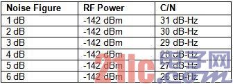
图16.C/N为噪声指数的函式

一般来说，接收器上的GPS译码芯片组，将得出定位作业所需的最小C/N比值。然而，又必须透过整组接收器的噪声指数，才能决定目前功率强度所能达到的C/N比值。因此，当测量灵敏度时，必须先了解定位作业所需的最小C/N比值。

其实有多种方法可测量灵敏度。如上表所示，RF功率与灵敏度具有直接相关性。因此，可根据现有的灵敏度功率强度，测量接收器的C/N比值;亦可根据不同的RF功率强度，得出系统灵敏度。

为了说明这点，则可注意RF信号功率与GPS接收器C/N比值，在不同功率强度之下的关系。下方测量作业所套用的激发，即忽略了第一组LNA而进行，且接收器的整体噪声指数约为8dB.而图17显示相关结果。

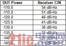
图17.接收器的C/N比值为RF功率的函式

如图17所示，此测量范例的RF功率与C/N比值，几乎是呈现完整的线性关系。而若使用高输入功率模拟C/N比值，将产生例外情况;接收器报表将出现可能的最大C/N值。然而，因为在任何条件下，进行实验的芯片组均不会产生超过54dB-Hz的C/N值，所以这些结果均属预期范围之中。

根据图7中所示RF功率与灵敏度之间的线性关系，其实仅需针对接收器模拟不同的功率强度，即可进行GPS接收器的生产测试作业。若接收器在-142dBm得出28dB-Hz的C/N值，则亦可于-136dBm得到34dB-Hz的C/N值。若特别注重测量速度，则可使用较高的C/N值，再从结果中推断出灵敏度的信息。

找出噪声指数

而由图17所示，接收器的噪声指数将直接与RF功率强度与载噪比互成比例。根据此关系，我们仅需针对RF功率强度与C/N进行关联性，即可测量芯片组的噪声指数。而此项测量中请注意，应以0.1dB为单位增加产生器的功率。由于NMEA-183协议所得到的卫星C/N值，是以最接近的小数字为准，因此在测量接收器C/N比值时，应估算噪声指数达1位数的精确度。范例结果如图18所示。

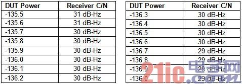
图18.DUT功率与接收器C/N的关联。

如图18所示，若RF功率强度处于-136.6dBm~-135.7dBm之间，则其C/N比值将维持于30dB-Hz.若以舍入法计算NMEA-183的数据时，则几乎可确定-136.1dBm功率强度将产生30.0dB-Hz的C/N比值无误。透过等式14，芯片组的噪声指数则为-174.0dBm+-136.1dBm+30.0dB-Hz=7.9dB.请注意，此计算是根据2组不确定性系数而进行：矢量信号发生器的功率不确定性，还有接收器所产生的C/N不确定性。

Solar Inverter

Solar Inverter,Solar Power Inverter,Sunpower Inverter,Residential Solar Inverter

Easun Power Technology Corp Limited , https://www.easun-power.com